07. DBSCAN Algorithm
DBSCAN Algorithm
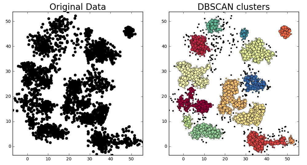
Original data on the left and clusters identified by the DBSCAN algorithm on the right. For DBSCAN clusters, large colored points represent core cluster members, small colored points represent cluster edge members, and small black points represent outliers.
The DBSCAN Algorithm
DBSCAN stands for Density-Based Spatial Clustering of Applications with Noise. This algorithm is a nice alternative to k-means when you don' t know how many clusters to expect in your data, but you do know something about how the points should be clustered in terms of density (distance between points in a cluster).
The DBSCAN algorithm creates clusters by grouping data points that are within some threshold distance d_{th} from the nearest other point in the data.
The algorithm is sometimes also called “Euclidean Clustering”, because the decision of whether to place a point in a particular cluster is based upon the “Euclidean distance” between that point and other cluster members.
You can think of Euclidean distance the length of a line connecting two points, but the coordinates defining the positions of points in your data need not be spatial coordinates. They could be defined in color space, for example, or in any other feature space of the data.
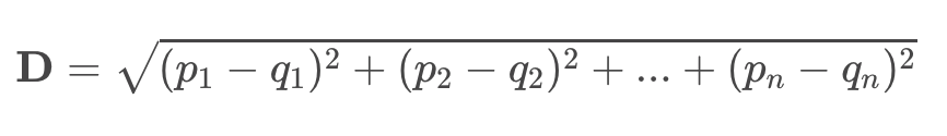
The Euclidean distance between points \bold{p} and \bold{q} in an n-dimensional dataset, where the position of \bold{p} is defined by coordinates (p_1, p_2, …, p_n) and the position of \bold{q} is defined by (q_1, q_2, …, q_n) then the distance between the two points is just:
DBSCAN Clustering Steps:
Suppose you have a set P of n data points p_1,p_2,…, p_n:
- Set constraints for the minimum number of points that comprise a cluster (
min_samples) - Set distance threshold or maximum distance between cluster points (
max_dist) - For every point p_i in P, do:
- if p_i has at least one neighbor within
max_dist:- if p_i's neighbor is part of a cluster:
- add p_i to that cluster
- if p_i has at least
min_samples-1 neighbors withinmax_dist:- p_i becomes a "core member" of the cluster
- else:
- p_i becomes an "edge member" of the cluster
- if p_i's neighbor is part of a cluster:
- else:
- p_i is defined as an outlier
- if p_i has at least one neighbor within
The above code is a bit simplified, to aid in a beginner's understanding of the algorithm. If you visited every data point at random, you would end up creating significantly more clusters than needed and would have to merge them somehow. We can avoid this by controlling the order in which we visit data points.
Upon creating a new cluster with our first qualifying data point, we will add all of its neighbors to the cluster. We will then add it's neighbor's neighbors, and their neighbors, until we have visited every data point that belongs to this cluster. Only after doing so, do we move on to choosing another data point at random. This way, we can guarantee that a cluster is complete, and there are no more points in the data set that belong to the cluster.
The full pseudo-code implementation of the DBSCAN algorithm can be found on the DBSCAN Wikipedia page.
Here's how the outcome looks visually for an example where min_samples = 4:
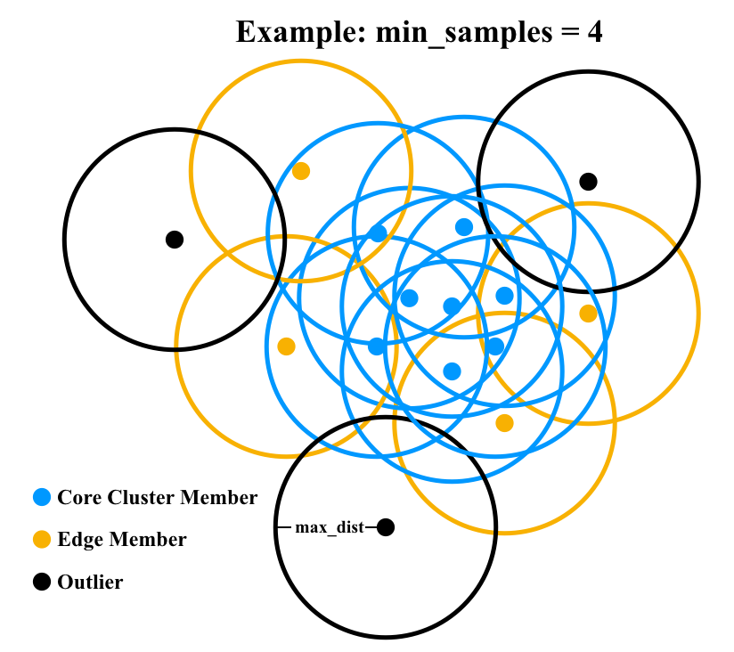
Blue points are core cluster members having at least three neighbors within max_dist (satisfying number of neighbors plus self >= min_samples. Yellow points are edge members having neighbors, but fewer than three. Black points are outliers having no neighbors.
It is once again worth visiting Naftali Harris' site to experiment with the interactive DBSCAN visualizer that he created.
While there, I recommend taking a look at Example A, as it demonstrates an interesting corner case where one data point falls into more than one cluster.
DBSCAN Playground
In this exercise I've built you a sandbox to play with the DBSCAN implementation from SciKit Learn. Let's take a look at the code used to implement this. First off, you'll be using the same cluster_gen() function as before in the k-means exercise. This time you can find it in the extra_functions.py tab below.
As far as new code goes, you've got the following:
# Import DBSCAN()
from sklearn.cluster import DBSCAN
After generating some data you're ready to run DBSCAN()
# Define max_distance (eps parameter in DBSCAN())
max_distance = 1.5
db = DBSCAN(eps=max_distance, min_samples=10).fit(data)
You can then extract positions and labels from the result for plotting:
# Extract a mask of core cluster members
core_samples_mask = np.zeros_like(db.labels_, dtype=bool)
core_samples_mask[db.core_sample_indices_] = True
# Extract labels (-1 is used for outliers)
labels = db.labels_
n_clusters = len(set(labels)) - (1 if -1 in labels else 0)
unique_labels = set(labels)
And the rest is just visualizing the result! Play around and see what happens as you vary parameters associated with the data you generate as well as varying max_distance and min_samples.
Start Quiz: